I wanted to start working on the motors to start controlling the players, but I have not really been satisified with the goal-checking mechanism (described in a previous post), because it depended too much on the performance of the webcam. In poor conditions, the camera records too few (useful) frames per seconds, which means that if you kick the ball very hard, there’s a good chance that the camera won’t catch it. This means that it will never detect the ball within the goal area (a precondition for detecting the goal), so a goal is never detected.
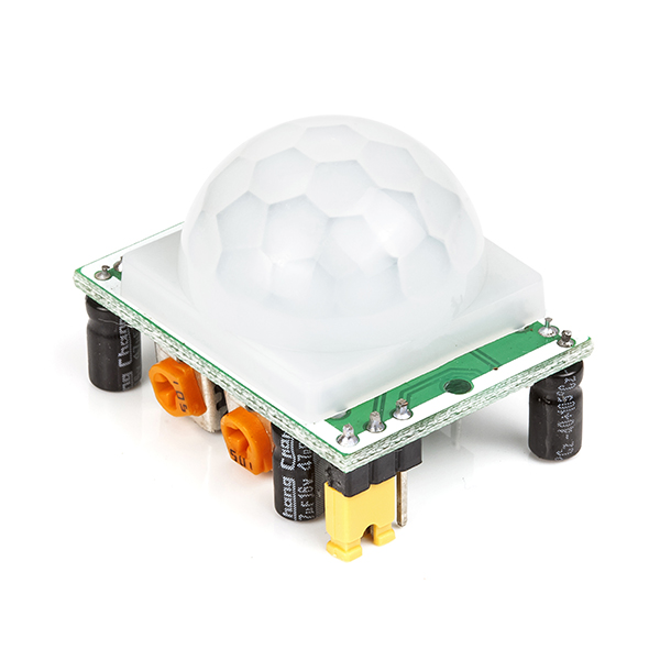
PIR Motion Sensor
First, I tried to use a PIR motion sensor. I wanted to place it near the goal area (outside the actual field), and if any motion is detected (i.e. when the ball is inside the goal), we infer that a goal is scored. However, it turned out to be too sensitive, because it also detected motion when the ball was moving between players (as it is visible through the goal). Again, I am no hardware expert, so it may have been obvious that it would not work. Anyway, I learned something.
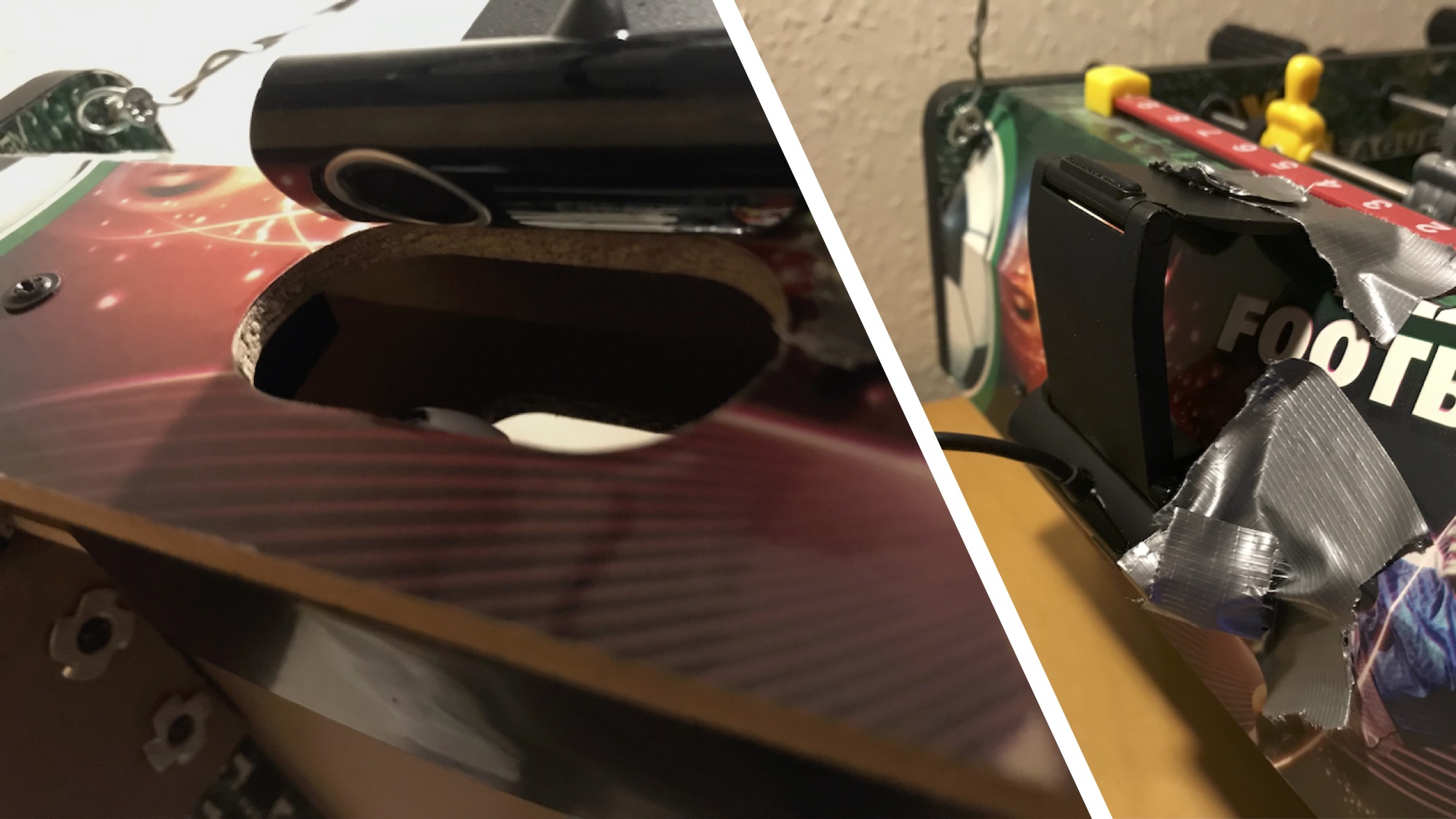
Webcam for motion detection
Instead, I figured I might be able to use another webcam, looking only at the goal. If motion is detected in the goal based on the camera feed, we infer that a goal is scored. I tried this and it turned out to actually work quite well.
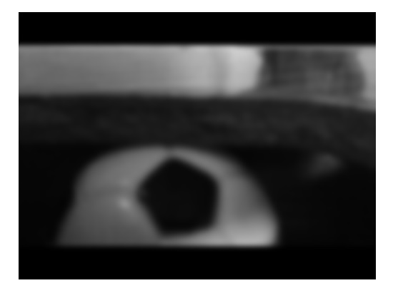
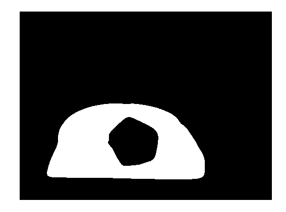
The implementation is based on this blogpost. The basic idea is to grab a frame as ‘baseline’, and then compare new frames to this. If there is a difference in pixels between the frames (and this difference is large enough), an object has been detected. In my case, this object would be the ball, and this means that a goal has been scored.
The algorithm for detecting a goal is then:
if motion detected and not goal_scored:
    if ball is not in field:
        goal_scored = True
else if ball is in field:
    goal_scored = False

if goal_scored:
    find scoring player using same method as before
See details of the implementation here. In other words, the main difference is that we do not check if the ball suddenly disappears, but instead rely solely on the motion detection from the new camera.
Conclusion
With this addition, I feel that the resulting application is more useful, because it is more precise in goal detection. There are still some issues with poor lighting conditions and a wobbly setup for the main camera, but all in all, it works quite well. The main issue is really that I only had one spare webcam, so I am only able to detect goals in one end of the field! … until I buy an extra, so it’s not that big an issue.
Now I can’t escape it anymore, so next big step will be to work on the motors and start controlling the players!
I have mentioned before that I have absolutely no experience in working with hardware, so I have decided to use Arduino to get something up and running fairly quickly.
Using an Arduino board, it is possible to interact with all sorts of hardware components through a serial interface. The board is programmed using the Arduino language, which is just a set of C/C++ functions, that are being called in the setup() and loop() functions of an application. The names of these functions make their purpose pretty clear.
I ordered a Starter Kit which includes the Arduino board itself, a lot of components to get started and a pretty good tutorial. After completing the first few tutorials (connecting LEDs and making them blink), I wanted to connect to the Table Soccer application.
Connecting to Python
As mentioned, the Arduino connects to a computer through a serial interface. This makes it pretty straightforward to communicate with it through Python. I used the pySerial library to access the serial port. It is very simple to use. For example, to send a string to the Arduino, the following code does the job:
import serial
s = serial.Serial("COM3", 9600)
s.write(b'Hello world!')
We connect to COM3 (as found in the device manager: ) and specify a baud rate of 96001. Reading the data on the Arduino is also easy enough:
void setup() {
  Serial.begin(9600);
  // initialize components
}

void loop() {
  while (Serial.available() > 0) {
    c = Serial.read();
    // do something with c
  }
}
Small steps, but steps nonetheless
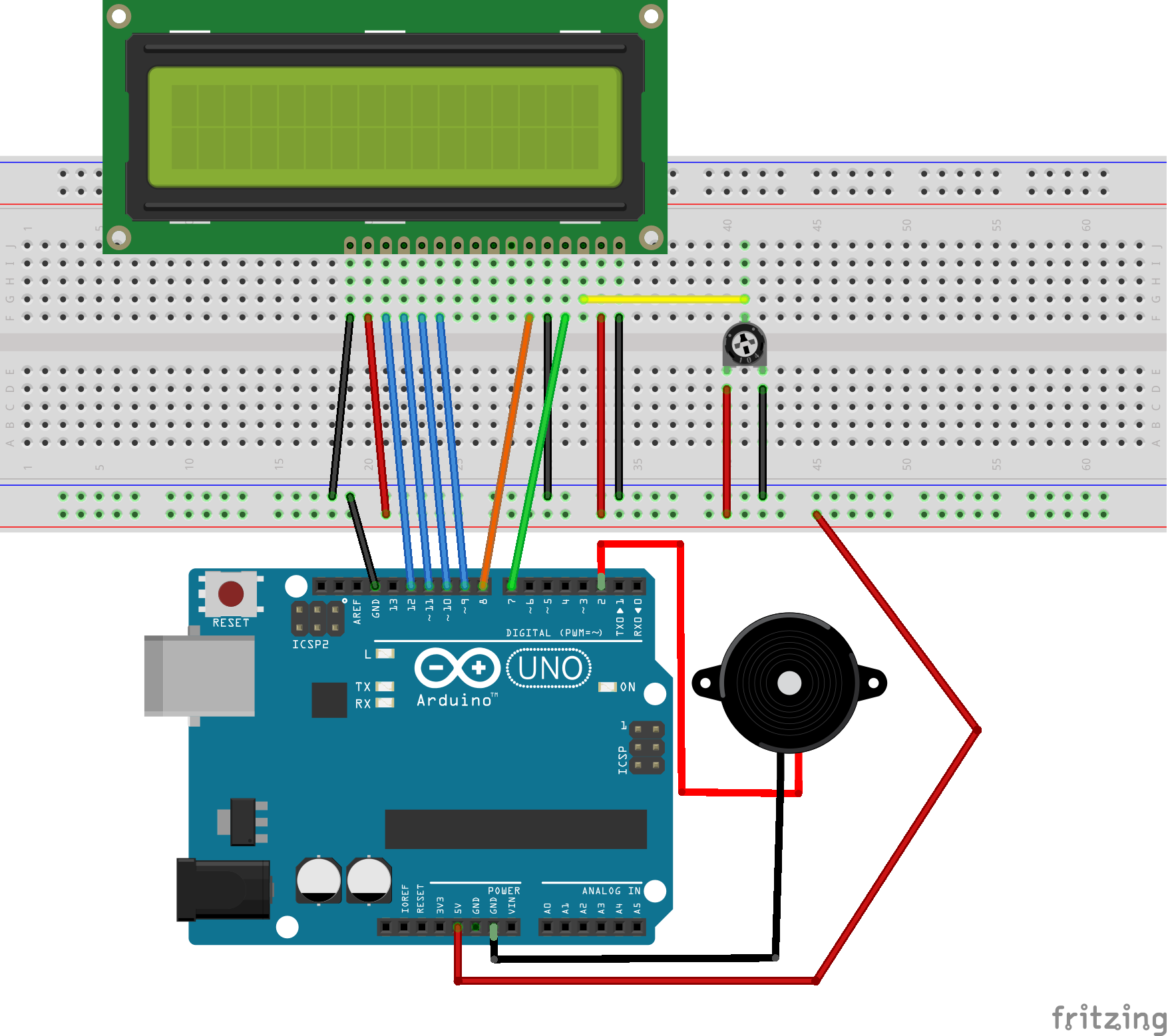
At some point, I will need to connect to some kind of motors that can control the players. To do so, I also need to attach the motors to the board. Since I am still new to Arduino, I wanted to try something simpler first, so I used an LCD and a buzzer to announce the goals of a match.
Using the very nice tutorial that came with the board, I was able to quickly setup an LCD that can write the scores. I also added a buzzer to play a sound when a goal is scored. The final schematics are as follows:
From the application, I can then send commands to the board through the serial port. It is done simply by sending strings, where the first character indicates the type of message and the rest of the string is the content. To write a message on the display, we can send the command Dtext and to play a sound, we use e.g. SA, where A is ‘away’, so we can play different sounds for each team. The implementation is found in this commit.
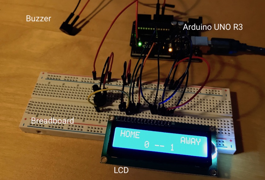
The result is then the following - extremely pretty - scoreboard:
Next steps
I have previously heard that Arduino makes it very easy to prototype, but I was surprised at how easy it was to have something working. Not just as a standalone application, but something that actually connects with the rest of the Table Soccer application!
Next, I will have to look into adding motors to the system now to get those players moving.
Footnotes
The baud rate specifies the number of bits per second that can be transmitted through the channel. ↩
In the previous post, I described how we could use the input data from the web-cam to start building a tablesoccer environment. This environment contains the current state of the real-life tablesoccer and it can be used to understand better what is happening. For example, we can compute different kinds of statistics, like ball possession, or keep track of goals scored. Later, the idea is to provide the environment to an agent controlling the players, so that it is able to make decisions and start playing autonomously.
There is still some way to go before we have a physical robot playing, and in this post I will describe the current state of the system and interface. You will see that we can now calculate ball possession (both per team and per player), can detect the rotation of each row of players and can detect when a goal is scored. This information will be quite useful for an agent, so it is a step in the right direction.
I will describe the implementation done in four parts:
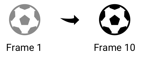
This is a pretty simple calculation, that can be done by comparing the location of the ball at two different times. For example, if the ball at frame 1 is at (0,0) and at frame 10 (now) is at (5,0), it has moved to the right, since the location is translated 5 units along the x-axis.
Implementation-wise, this means that the environment will keep track of the ball’s previous locations. Every time we need to calculate the direction, we look at where the ball was 10 frames ago, and where it is now. We then calculate the change on each axis.
prev = self.history[-10]["position"]
this = self.history[-1]["position"]

dX = prev[0] - this[0]
dY = prev[1] - this[1]
We define a significant movement as a movement of more than 10 pixels, so if the magnitude of dX or dY is greater than 10, there is a movement on that axis. The sign of the number tells us which of way the ball has moved (e.g. we move to the left on the x-axis, if the number is less than zero). If there is a significant movement in both directions, the direction will be of the form ‘DirectionY-DirectionX’, for example: ‘Down-Right’.
Calculate player rotation
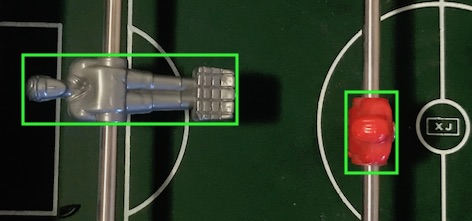
Everything we see is from above, so we need a way to calculate rotation. Looking at a picture of the bounding boxes may help us in the right direction:
As we can see, a player is rotated if the width of the bounding box is greater than the height, and vice versa. We say that the player is 0% rotated when standing (right player), and 100% rotating when lying (left player). This, however, does not tell us specifically what the ratio should be when the player is 0% or 100% rotated.
One approach to calculate this is to calibrate: we do a full rotation of the row, and the application detects the minimum and the maximum ratios. These will be the 0% and 100%, respectively. However, in my current setup, I don’t want to have to calibrate before playing (after all, it should work for my kids), so I defined the minimum and maximum ratio by trial and error1.
There is an uncertainty in the approach of using the bounding box: The camera films from a single spot in the middle of the field, so when the players are actually 0% rotated, the camera will detect a slight angle, and believe that they are 10-15% rotated. I am not sure whether this will be a problem, but we will have to see, and eventually revisit this.
Having defined the minimum and maximum ratio, the calculation of the rotation is very simple:
Before we can calculate the ball possession, we need to define what it means to possess the ball. We here propose that a player possesses the ball if it is within the player’s reach. That is, we define an area around the player (the area he can reach), and then we can calculate how much time the ball spends in that area.
We do this by keeping track of which player has possession of the ball in each frame in a ‘possession-table’. For each player, the possession-table will contain the number of frames in which the player possessed the ball. We can then calculate the possession for a player as # frames with possession / # total frames.
We consider the area of reach as a rectangle around the player. We thus need to calculate if the position of the ball is within this rectangle. For each row, we then calculate (for each player) whether the ball is within reach. If so, we increment the possession-table by one for that player.
def calculate_possession(self, ball_position):
    for i, player in enumerate(self.players):
        reach_x_start = player[0] - REACH_WIDTH / 2
        reach_x_end = player[0] + REACH_WIDTH / 2
        reach_y_start = player[1] - REACH_HEIGHT / 2
        reach_y_end = player[1] + REACH_HEIGHT / 2

        ball_x = ball_position[0]
        ball_y = ball_position[1]

         if reach_x_start < ball_x < reach_x_end
                and reach_y_start < ball_y < reach_y_end:
            self.possession[i] += 1
            break
To calculate team possession, we initialize the game with a configuration of the board, containing information about number of rows, number of players in each row, and the team each row belongs to:
The team’s possession is then # frames with possession for players in team / # total frames. We now have the possession for both team and players:
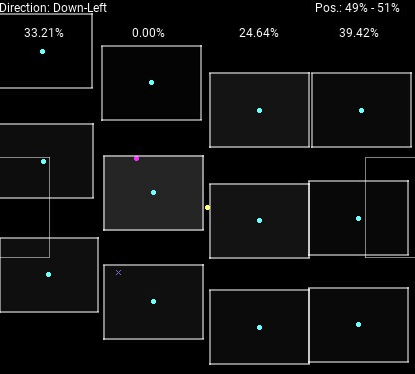
The teams’ possession are shown in the top-right corner, and the each player’s possession is indicated by the opacity of the ‘reach’ rectangle around the player. This visualization also shows the rotation of each row (percentages in the top) and the current direction of the ball.
Detect goals
You may have noticed a small cross in the image above. This actually indicates that a goal was scored from that position. Not only do we detect if a goal has been scored, we also attempt to figure out from which position and by which player.
Inspired by another Table Soccer project, TableSoccerCV, the intuition behind goal detection is to (1) detect that the ball is close to the goal and (2) detect that the ball has now disappeared. If it has disappeared, and was close to the goal, odds are that a goal was scored.
In each game loop, we do as follows:
if ball is in area in front of goal
    check_for_goal <- true

if check_for_goal is true
    if ball has disappeared
        increment frames_without_ball by 1
        if frames_without_ball > 15
            GOAL!!
In other words, when the ball has not been seen for 15 frames (but was seen outside the goal just before), this counts as a goal. The most prominent issue with this, is that it is possible for the ball to be hidden behind or below the goalkeeper. This will result in a false detection of a goal.
When a goal is scored, we then use the history of the ball’s location to figure out the scoring position. We do this by traversing back in history, until the direction of the ball changes. The intuition is that this is the point in time when the shot was performed. It does not work perfectly, e.g. if the ball bounces of another player before entering the goal, but provides an estimate.
We also want to know which specific player scored, so we keep a history of the players’ position together with the ball. When we know from where the goal was scored, we can simply find the player closest to the ball at that time.
for r, row in enumerate(self.player_history[i]):
    for p, player in enumerate(row.get_players()):
        dist = np.linalg.norm(np.array(pos) - np.array(player[0:2]))
        if dist < min_dist:
            min_dist = dist
            player_info["row"] = r
            player_info["position"] = p
Visualization
We now have information about the score, goals and ball possession. Using Flask (as also mentioned in the previous post) we can create a better interface to show and control the application form a browser. We get the current stats using an API endpoint:
The web application fetches data from this endpoint every few seconds and populates the model in the webpage. I have chosen to use Knockout.js because of its simplicity and possibility to do declarative bindings, making the implementation of the UI very straightforward. I can simply specify the scores as follows:
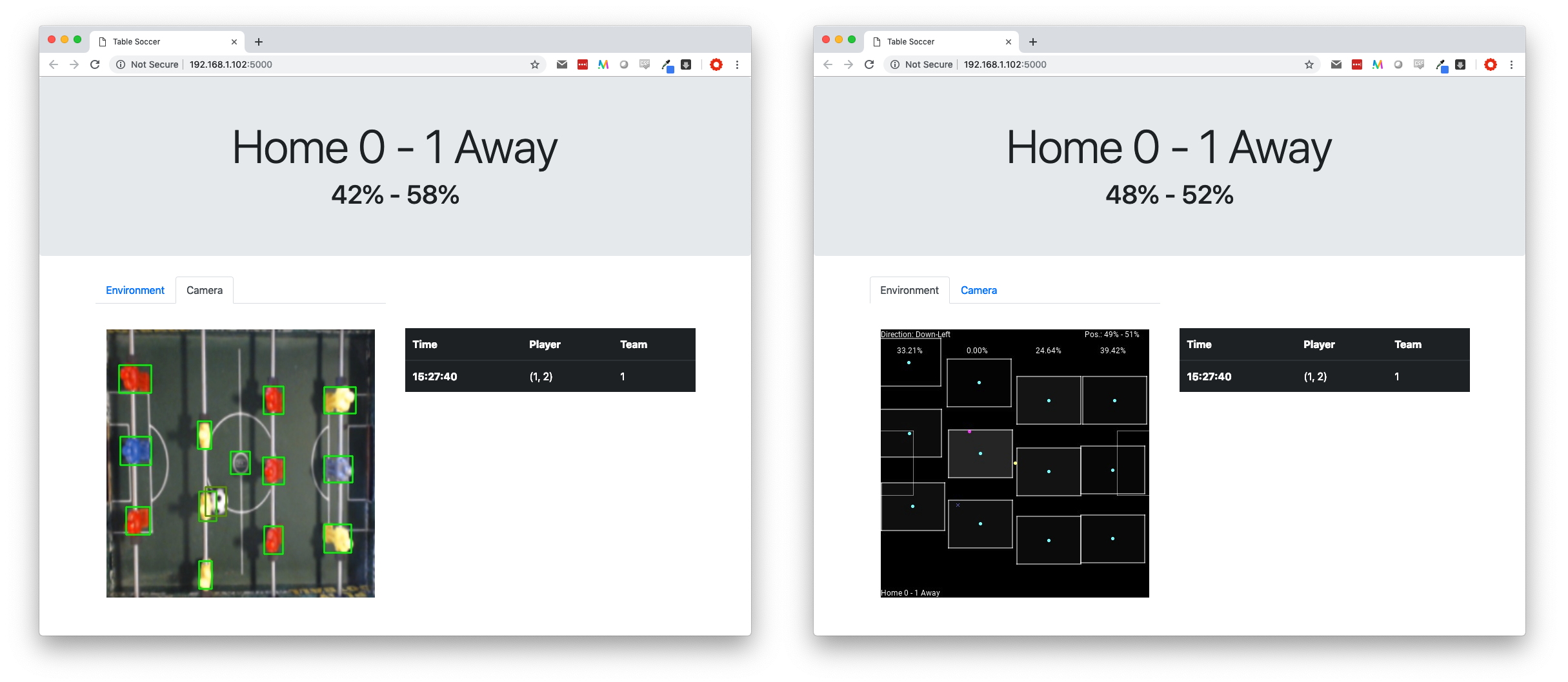
The result is shown below. On the left side, we see the transformed view of the webcam and on the right side, we see the environment representation of the field.
Next steps
Now I can’t postpone it anymore - I am going to start working on the robot. Since I have not worked with hardware much before, the next post will probably be about some of the exploration I am doing in that field.
Footnotes
I am aware that we could use the predefined values, and still calibrate, but for now I will just stick to the calculated values as it seems to be fairly accurate. Of course, if this should be extended to support other tables, we would need some calibration mechanism. ↩
In this post, I describe how to use the input from the model created in the previous post. We have a number of detected objects, including their class, location and size. We would like to use this information to track things like scoring a goal, ball possession, ball speed, etc.
The first issue is to get data into Python from the webcam fast enough. Using OpenCV, it is quite easy to read from the webcam:
However, this method is very inefficient, because it is running on the main thread, which means that polling the webcam is blocking the rest of the application1. We can move it to a separate thread using features of the imutils package:
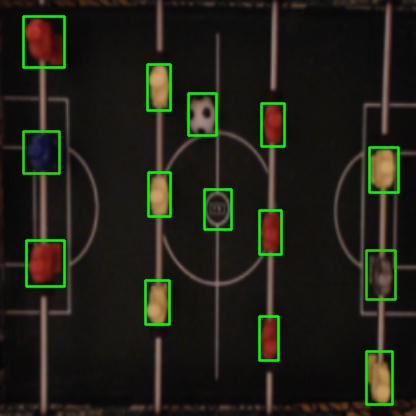
Now that I have a frame, detecting objects is straightforward using the darknet python library2:
result = darknet.performDetect(frame, makeImageOnly=True, configPath=config, weightPath=weights, metaPath=data)
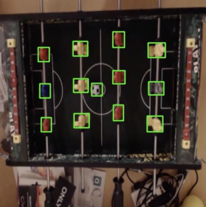
This gives us an image I’ve shown before:
The image is not all - we also get a list of detections containing the class, location and size in the format (<class>, <confidence>, (<x>,<y>,<width>,<height>)):
Using this, we can build a representation of the environment which can then be used to calculate statistics, for training the and maybe for visualizing some interesting statistics later.
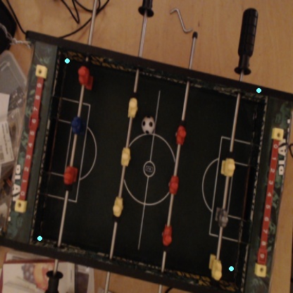
Problem: It’s all rotated
There is a potential problem with my setup. Because of the way the camera is installed, we cannot guarantee that the view from above will always show the field consistently with no rotation. When implementing an environment, we would like to be able to assume, e.g. that all players in one row are located exactly beneath each other (i.e. having the same x coordinate), and that the two goals are located directly opposite each other (having coordinates (0, <y>) and (<field length>, <y>), respectively).
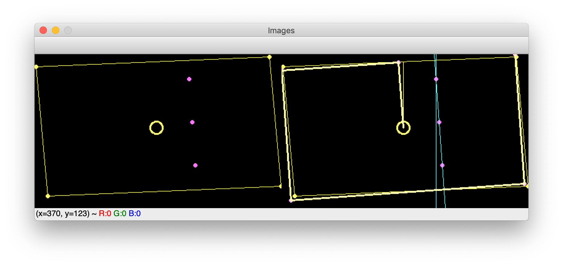
Using a few simple calculations, we are able to estimate the location of the corners of the actual board. The following will be used:
Field center location and size
One row of players’ locations
Using the size of the center, we can calculate the size of the entire table (since we know the physical size of the center and of the entire table). We can estimate the angle of rotation by using a row of players.
Simply put, we calculate the angle between the vector going through the players in the row (the actual rotation) and a vertical vector (the assumed rotation). Using that, we can find the midpoint of the side of the field. Since we know now the angle of rotation and the length of the sides, it is straightforward to estimate the corners’ location.
The figure shows on the left side a representation of a rotated table with a row of players. On the right side, we show the calculated vectors and how they estimate the corner location of the actual table.
Transforming positions
Using the coordinates of the corners, all that is left to do is to transform the detected locations into the new coordinate system. However, I have chosen a bit different method. I do a four-point perspective transformation3, which takes as input the image and the four calculated corners. As an output, we get a transformed image that only contains the field (within the corners) and is warped into a rectangular shape. We thus obtain a consistent image containing only the field. To obtain the location of ball and players, we use Yolo once again and voila:
My reason for doing like this is:
We only detect the corners once (assuming that the camera does not move during a match)
The rest of the time, we use OpenCV to get a consistent picture of the field, ensuring that no erroneous detections will be made outside the field (e.g. a hand being confused with a player)
There may be many other ways to solve this, but it was a fun little exercise and the result is satisfactory.
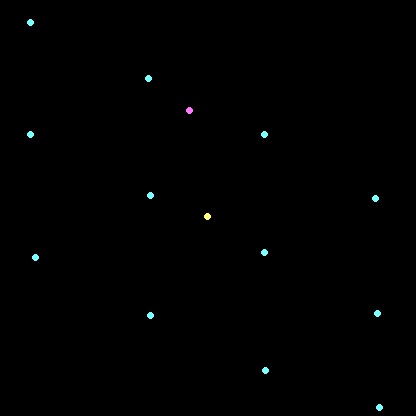
The final environment
Using this method, we now have a consistent representation of the field and an environment which at all times contains updated information about ball and player location:
Using Flask, I created a small web-application to show the stream and send commands to the system. I created a route for publishing the feed using Motion JPEG4, which will take the latest image produced from the system (e.g. the environment or the raw detections) and add it to the stream. Further, to allow recalculation of the corners on demand, it is possible to add a route to do so.
def gen(image):
    while True:
        frame = d.snapshots.get(image)
        if frame is not None:
            _, jpeg = cv2.imencode('.jpg', frame)
            yield (b'--frame\r\n'
                   b'Content-Type: image/jpeg\r\n\r\n' + jpeg.tobytes() + b'\r\n\r\n')


@app.route('/video/<feed>')
def video(feed):
    return Response(gen(feed),
                    mimetype='multipart/x-mixed-replace; boundary=frame')


@app.route('/recalculate')
def recalculate():
    d.schedule_recalculation()

    return "ok"
Next steps
With a consistent environment, the next step will be to calculate a few simple statistics like ball possession, goals and ball speed and present those in the web-application.
The next step after that is to start building the actual robot! I am very eager to begin, but a start, I will probably add an interface in the web-application to control the robot, just to verify that everything works. After that, the real fun begins: build an autonomous controller that can actually play (and hopefully well!).
In this post, I describe how I have trained a model that can detect the different parts of a tablesoccer table. The title implies that this is being done by building on previous achievements. This is what transfer learning can help us do.
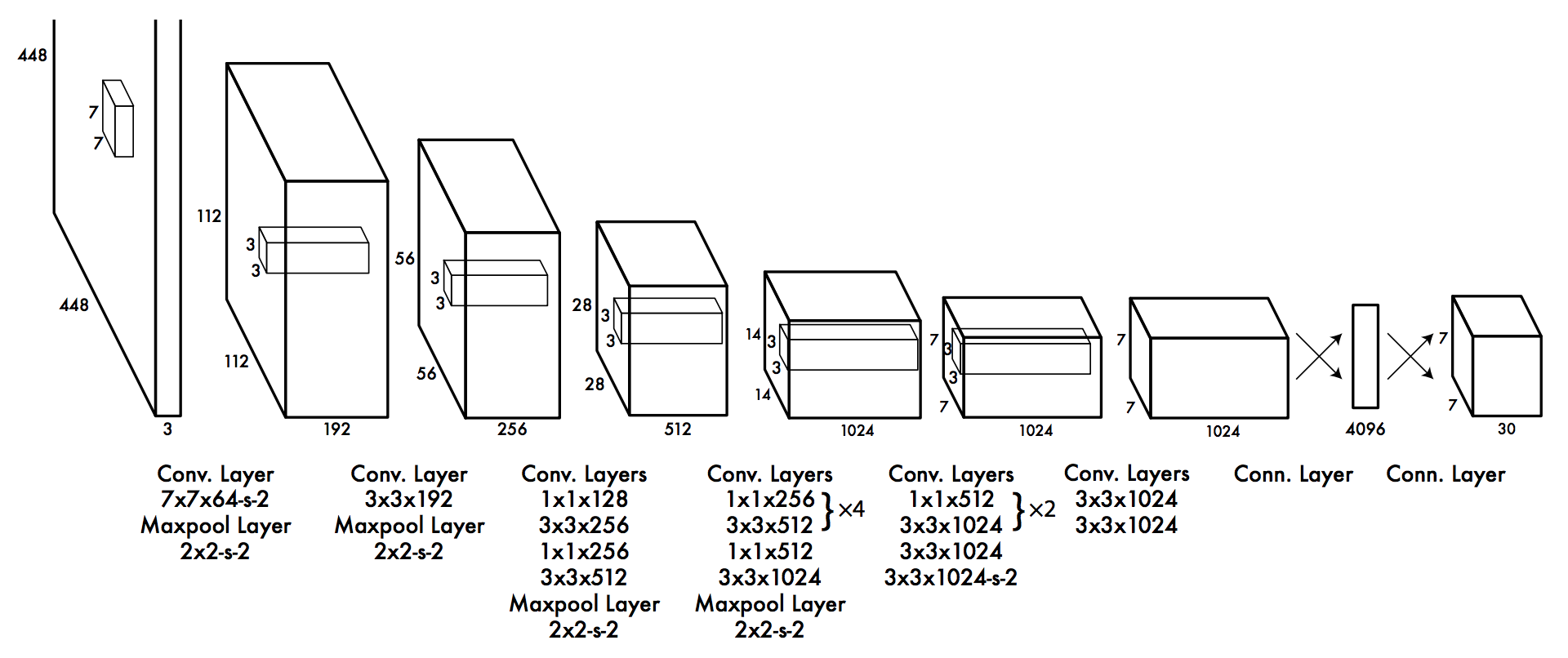
Object detection and localization can be very powerful, but it requires large amounts of data to get to a point where it is actually useful and accurate. Since we want to create a model that can recognize tablesoccer with high accuracy, we would need a very large dataset of images in different situations to be used in the training.
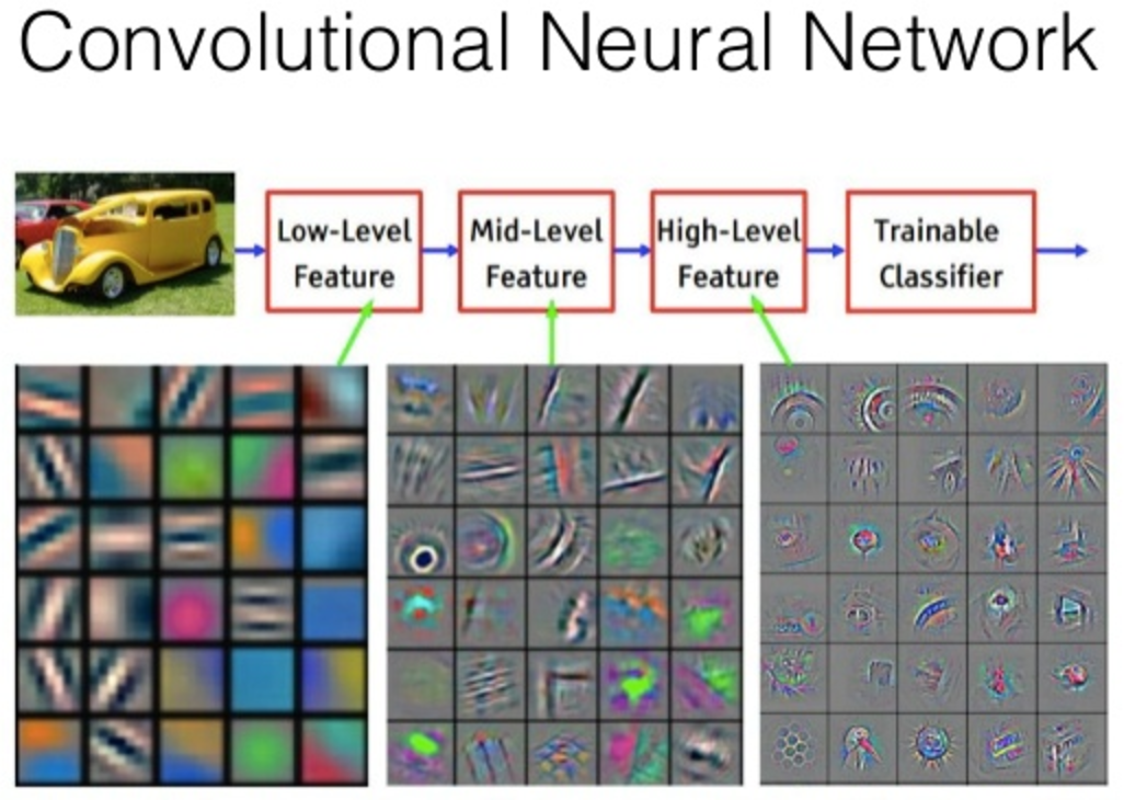
The reason we need a very large dataset is that in order for the model to learn good weights, it needs to see a lot of examples. The YOLO architecture is shown in the figure above. The convolutional layers will learn to detect features of an image, and as mentioned in the previous post, the first layers will learn to detect features such as edges or colors, while later layers will be able to detect more complex features such as ears, faces or even specific objects, like a car (of course, the specific features they can detect depend on the training data used).
Essentially, this means that if we train a model from scratch, we will first need to learn to detect simple features before moving to the more complex ones, like the players in tablesoccer. What transfer learning does, is to remove the output layer and the weights to that layer, and replace it with a new output layer that can detect our domain-specific objects. We can then retrain the network with our own training data. We thus build on top of a network that can already detect complex features, and rewire it to be able to use those features to detect objects in our domain.
The Darknet implementation that I am using supports transfer learning, which means that we can use the Yolo-tiny model mentioned in the previous post and train it to track tablesoccer.
Visualizing the layers
As a side note (because I think it is cool), it is possible to visualize what a network ‘sees’ at each layer by using a DeConvNet. A DeConvNet performs (roughly speaking) the operations of a CNN in reverse. This means that it can take activations of a specific layer in a CNN and pass these as input to the DeConvNet. The output of the DeConvNet is an image in the same space as the original input image to the CNN.
In the image above, which is created using a DeConvNet, we clearly see a increase in complexity from the first layer to the last. In the first layer, we see low-level features such as edges and colors, while the last layer contains things like a honeycomb pattern and an eye.
Of course, in our domain, we probably won’t see honeycombs, eyes or other complex patterns, but by being able to detect complex features, the network will be better at distinguishing different patterns. Hopefully, this will also result in a more accurate tracking in this case.
Getting training data
To train the Yolo model, I have to provide the network with lots of training examples. These examples will be images of the tablesoccer table that are annotated with bounding boxes around the objects that the network should learn to detect. The annotations are created in plain text files with one bounding box per line. The format is: <object-class> <x> <y> <width> <height>. In our case, the object classes are:
0: Ball
1: Player
2: Table center
I have chosen to detect the table center as well, because if we know the size and position of it, we can calculate the size of the table. This makes it possible to focus on the actual field and not any movement outside of it. I will get back to this in a later post.
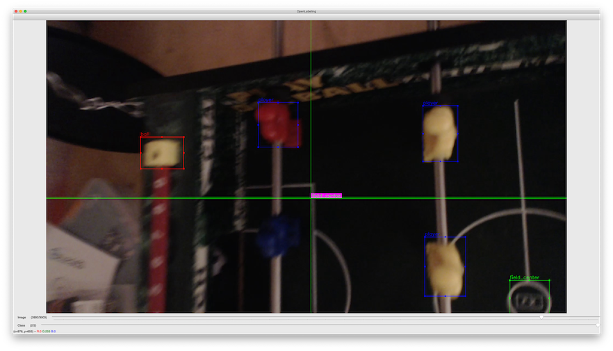
Creating these files manually is a tedious process, so I used OpenLabeling which is a GUI application that makes annotating much easier.
I recorded a few videos of the table while playing.
The videos were put into the input/ folder of OpenLabeling.
OpenLabeling then automatically converted the video into individual frames:
 Converting video to individual frames...
100%|████████████████████████████████████████| 657/657 [00:03<00:00, 169.85it/s]
I annotated each frame manually in the GUI.
Need for Speed
I initially only labeled 100 images, and then used some tricks to speed up the creation of training data. First, OpenLabeling comes with a feature to predict the next frames’ labels. After labeling an image, we can ask the application to predict the next frames. It will then try to find the same objects in the next few frames using OpenCV. It worked quite well, but it was still largely a manual task.
The second trick is to use a trained model to label new images. So once I had the first few hundred labels, I trained a first version of the network. It actually performed pretty alright, probably due to the fact that the environment doesn’t change much. However, the average loss never came down below 2, and I wanted to get it below 1 (as recommended by the Darknet authors).
Pseudo-labeling is very straightforward. Provide Darknet with the model and ask it test on a bunch of images. The key is to include the flag -save_labels to save the detected bounding boxes.
I took the generated labels and put them into the output/YOLO_darknet/ folder of OpenLabeling. However, it turns out that OpenLabeling primarily uses the Pascal VOC format (but outputs the Darknet format as well), so I created a utility script to convert the files into the correct format.
The pseudo-labeling worked quite well for the most static parts of the video, but to add some distortion and noise I moved the camera around a bit. In that case, it sometimes detected a ball where there wasn’t any (the red bounding box). In many cases, it had a hard time finding the blue player. This could most likely be mitigated by turning on more light in the room, but I would rather have a more robust model.
I did the pseudo-labeling in a few iterations. After the first iteration, I had 400 training examples. I then retrained (and improved) the model, so I did a pseudo-labeling of the rest of the training examples. I finally had a dataset with ~3.000 examples.
Training the model
To train the mode, we first need to get the partial model from the full model (i.e. without the last layer):
We create a data-file to configure the training and validation sets, number of classes, etc:
classes= 3
train  = train.txt
valid  = test.txt
names  = tablesoccer.names # the class names
backup = weights/
To start the training, we thus have to start Darknet with our own configuration and the partial model. However, I experienced from time to time that Darknet crashed without any error messages. I don’t want to spend to much time debugging things like this, so I ‘fixed’ it by using the fact that Darknet creates an updated ‘weights’ file at every 100 iterations. The fix was an infinite loop:
Not very elegant, but it got the job done and I was able to train for 25.000 iterations and the average loss stabilized below 1.
Evaluation
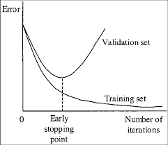
Darknet also saves weights every 1.000 iterations. This is useful to make sure that the final weights we choose are not overfitted to the training set.
The image shows the early stopping point, which is the point where the validation error is at its minimum. In other words, after this point, the network is being overfitted to the training data: the training error decreases, but the validation error increases.
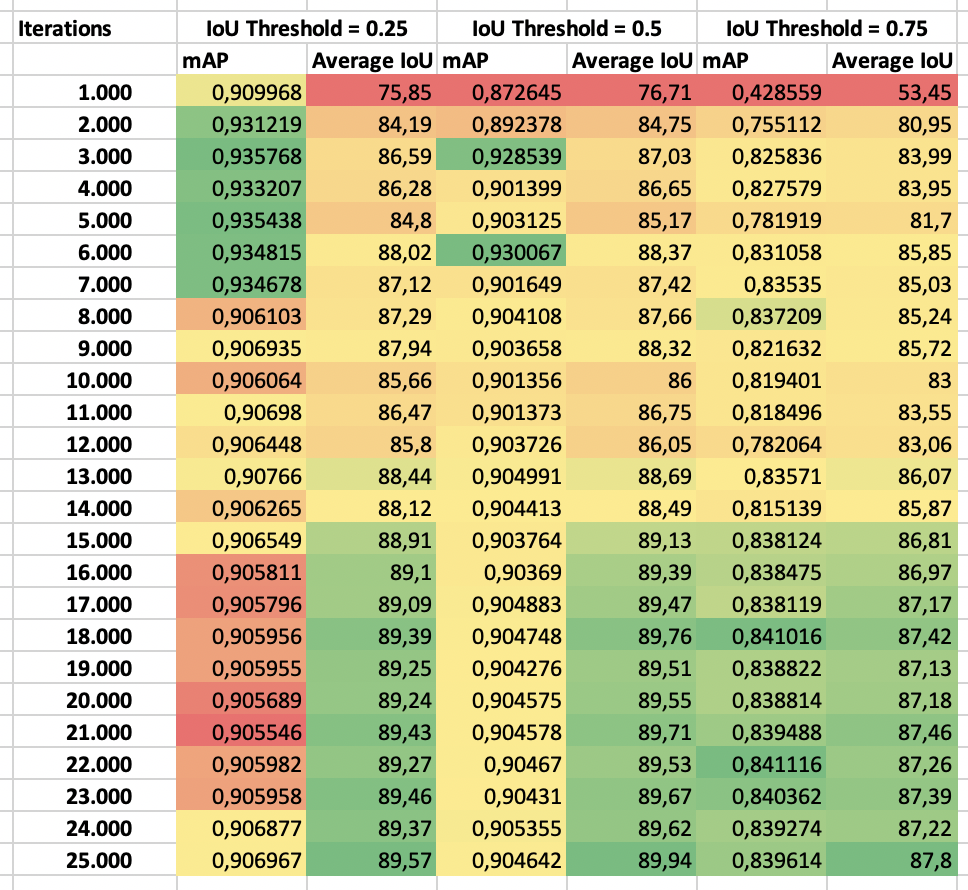
I calculated the mAP for each of the saved weights:
for /f %%f in ('dir /b weights') do (
    echo %%f >> eval.txt
    darknet.exe detector map tablesoccer.data yolov3-tablesoccer.cfg weights/%%f -iou_thresh 0.5 >> eval.txt
)
We can then evaluate the mAP for each set of weights and choose the weights with the highest mAP:
We see that with an IoU threshold of 50%, the mAP is highest at iteration 6.000. It is, however, pretty stable at around 0.9 throughout the training.
Since the calculation of mAP is based on the average precision of each class, we can also check if a specific class is harder to detect than others. It turns out that the ball is the hardest to detect:
class_id = 0, name = ball, ap = 70.56 %
class_id = 1, name = player, ap = 90.84 %
class_id = 2, name = field_center, ap = 90.91 %
This is as expected, as the ball is the most dynamic part of the environment, but it would be good to increase the average precision.
Peeking into the brain
Here is a short video of how well it is able to track the players and ball using the model we chose above:
We see the same pattern here: the ball is hard to detect, especially when it is located close to the players.
Next steps
We have a network that can detect the players and the ball, but there is still room for improvement. In a later post, I will try to improve the accuracy by adding more specific training examples for the tough spots, and see how it improves.
Before that, though, I want to implement an application that can track the position of the ball using this model and provide some simple statistics of the game. Stay tuned!
 ) and specify a baud rate of 9600