Standing on the Shoulders of Giants
27 Feb 2019In this post, I describe how I have trained a model that can detect the different parts of a tablesoccer table. The title implies that this is being done by building on previous achievements. This is what transfer learning can help us do.
Object detection and localization can be very powerful, but it requires large amounts of data to get to a point where it is actually useful and accurate. Since we want to create a model that can recognize tablesoccer with high accuracy, we would need a very large dataset of images in different situations to be used in the training.
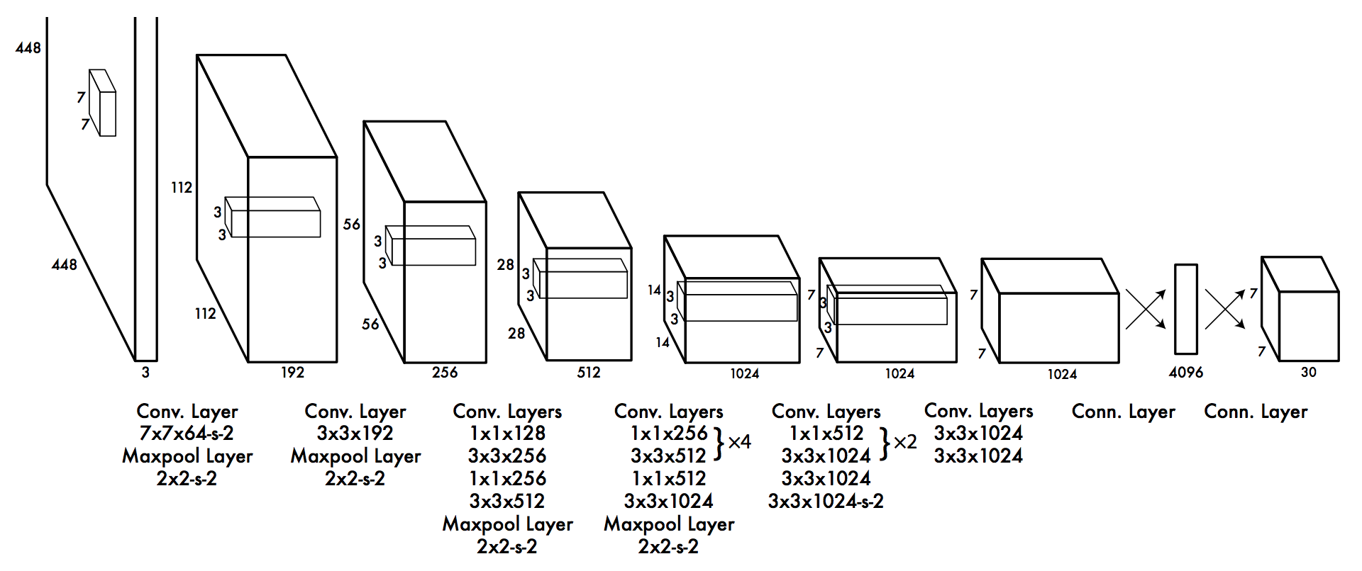
The reason we need a very large dataset is that in order for the model to learn good weights, it needs to see a lot of examples. The YOLO architecture is shown in the figure above. The convolutional layers will learn to detect features of an image, and as mentioned in the previous post, the first layers will learn to detect features such as edges or colors, while later layers will be able to detect more complex features such as ears, faces or even specific objects, like a car (of course, the specific features they can detect depend on the training data used).
Essentially, this means that if we train a model from scratch, we will first need to learn to detect simple features before moving to the more complex ones, like the players in tablesoccer. What transfer learning does, is to remove the output layer and the weights to that layer, and replace it with a new output layer that can detect our domain-specific objects. We can then retrain the network with our own training data. We thus build on top of a network that can already detect complex features, and rewire it to be able to use those features to detect objects in our domain.
The Darknet implementation that I am using supports transfer learning, which means that we can use the Yolo-tiny model mentioned in the previous post and train it to track tablesoccer.
Visualizing the layers
As a side note (because I think it is cool), it is possible to visualize what a network ‘sees’ at each layer by using a DeConvNet. A DeConvNet performs (roughly speaking) the operations of a CNN in reverse. This means that it can take activations of a specific layer in a CNN and pass these as input to the DeConvNet. The output of the DeConvNet is an image in the same space as the original input image to the CNN.
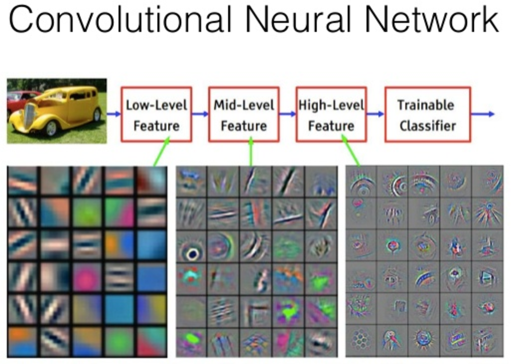
In the image above, which is created using a DeConvNet, we clearly see a increase in complexity from the first layer to the last. In the first layer, we see low-level features such as edges and colors, while the last layer contains things like a honeycomb pattern and an eye.
Of course, in our domain, we probably won’t see honeycombs, eyes or other complex patterns, but by being able to detect complex features, the network will be better at distinguishing different patterns. Hopefully, this will also result in a more accurate tracking in this case.
Getting training data
To train the Yolo model, I have to provide the network with lots of training examples. These examples will be images of the tablesoccer table that are annotated with bounding boxes around the objects that the network should learn to detect. The annotations are created in plain text files with one bounding box per line. The format is: <object-class> <x> <y> <width> <height>. In our case, the object classes are:
- 0: Ball
- 1: Player
- 2: Table center
I have chosen to detect the table center as well, because if we know the size and position of it, we can calculate the size of the table. This makes it possible to focus on the actual field and not any movement outside of it. I will get back to this in a later post.
An example of an annotation file:
0 0.59765625 0.7511737089201878 0.0484375 0.07511737089201878
1 0.36328125 0.38967136150234744 0.0421875 0.0892018779342723
1 0.37578125 0.18309859154929578 0.0515625 0.09389671361502347
1 0.3515625 0.5915492957746479 0.046875 0.08450704225352113
1 0.7328125 0.37910798122065725 0.115625 0.09154929577464789
1 0.69375 0.7582159624413145 0.115625 0.12206572769953052
1 0.71015625 0.573943661971831 0.1171875 0.11032863849765258
1 0.5640625 0.2734741784037559 0.059375 0.10093896713615023
1 0.546875 0.47769953051643194 0.05625 0.1056338028169014
1 0.53203125 0.6725352112676056 0.0609375 0.09154929577464789
1 0.19765625 0.10093896713615023 0.0984375 0.09389671361502347
1 0.1796875 0.5093896713615024 0.096875 0.08450704225352113
1 0.1890625 0.3086854460093897 0.096875 0.08215962441314555
2 0.4640625 0.4072769953051643 0.04375 0.07276995305164319
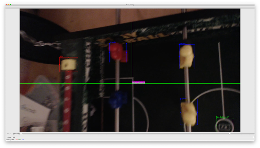
Creating these files manually is a tedious process, so I used OpenLabeling which is a GUI application that makes annotating much easier.
- I recorded a few videos of the table while playing.
- The videos were put into the
input/folder of OpenLabeling. - OpenLabeling then automatically converted the video into individual frames:
Converting video to individual frames... 100%|████████████████████████████████████████| 657/657 [00:03<00:00, 169.85it/s] - I annotated each frame manually in the GUI.
Need for Speed
I initially only labeled 100 images, and then used some tricks to speed up the creation of training data. First, OpenLabeling comes with a feature to predict the next frames’ labels. After labeling an image, we can ask the application to predict the next frames. It will then try to find the same objects in the next few frames using OpenCV. It worked quite well, but it was still largely a manual task.
The second trick is to use a trained model to label new images. So once I had the first few hundred labels, I trained a first version of the network. It actually performed pretty alright, probably due to the fact that the environment doesn’t change much. However, the average loss never came down below 2, and I wanted to get it below 1 (as recommended by the Darknet authors).
Pseudo-labeling is very straightforward. Provide Darknet with the model and ask it test on a bunch of images. The key is to include the flag -save_labels to save the detected bounding boxes.
darknet.exe detector test tablesoccer.data yolov3-tablesoccer.cfg
    weights/yolov3-tablesoccer_last.weights -thresh 0.25
    -dont_show -save_labels < new_examples.txt
I took the generated labels and put them into the output/YOLO_darknet/ folder of OpenLabeling. However, it turns out that OpenLabeling primarily uses the Pascal VOC format (but outputs the Darknet format as well), so I created a utility script to convert the files into the correct format.
The pseudo-labeling worked quite well for the most static parts of the video, but to add some distortion and noise I moved the camera around a bit. In that case, it sometimes detected a ball where there wasn’t any (the red bounding box). In many cases, it had a hard time finding the blue player. This could most likely be mitigated by turning on more light in the room, but I would rather have a more robust model.
I did the pseudo-labeling in a few iterations. After the first iteration, I had 400 training examples. I then retrained (and improved) the model, so I did a pseudo-labeling of the rest of the training examples. I finally had a dataset with ~3.000 examples.
Training the model
To train the mode, we first need to get the partial model from the full model (i.e. without the last layer):
darknet.exe partial cfg/yolov3-tiny.cfg yolov3-tiny.weights yolov3-tiny.conv.15 15
We create a data-file to configure the training and validation sets, number of classes, etc:
classes= 3
train  = train.txt
valid  = test.txt
names  = tablesoccer.names # the class names
backup = weights/
To start the training, we thus have to start Darknet with our own configuration and the partial model. However, I experienced from time to time that Darknet crashed without any error messages. I don’t want to spend to much time debugging things like this, so I ‘fixed’ it by using the fact that Darknet creates an updated ‘weights’ file at every 100 iterations. The fix was an infinite loop:
:start
if exist weights/yolov3-tablesoccer_last.weights (
    darknet.exe detector train tablesoccer.data yolov3-tablesoccer.cfg weights/yolov3-tablesoccer_last.weights -map
) else (
    darknet.exe detector train tablesoccer.data yolov3-tablesoccer.cfg %DARKNET_DIR%/yolov3-tiny.conv.15 -map
)
goto start
Not very elegant, but it got the job done and I was able to train for 25.000 iterations and the average loss stabilized below 1.
Evaluation
Darknet also saves weights every 1.000 iterations. This is useful to make sure that the final weights we choose are not overfitted to the training set.
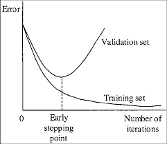
The image shows the early stopping point, which is the point where the validation error is at its minimum. In other words, after this point, the network is being overfitted to the training data: the training error decreases, but the validation error increases.
I calculated the mAP for each of the saved weights:
for /f %%f in ('dir /b weights') do (
    echo %%f >> eval.txt
    darknet.exe detector map tablesoccer.data yolov3-tablesoccer.cfg weights/%%f -iou_thresh 0.5 >> eval.txt
)
We can then evaluate the mAP for each set of weights and choose the weights with the highest mAP:
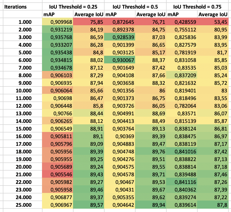
We see that with an IoU threshold of 50%, the mAP is highest at iteration 6.000. It is, however, pretty stable at around 0.9 throughout the training.
Since the calculation of mAP is based on the average precision of each class, we can also check if a specific class is harder to detect than others. It turns out that the ball is the hardest to detect:
class_id = 0, name = ball, ap = 70.56 %
class_id = 1, name = player, ap = 90.84 %
class_id = 2, name = field_center, ap = 90.91 %
This is as expected, as the ball is the most dynamic part of the environment, but it would be good to increase the average precision.
Peeking into the brain
Here is a short video of how well it is able to track the players and ball using the model we chose above:
We see the same pattern here: the ball is hard to detect, especially when it is located close to the players.
Next steps
We have a network that can detect the players and the ball, but there is still room for improvement. In a later post, I will try to improve the accuracy by adding more specific training examples for the tough spots, and see how it improves.
Before that, though, I want to implement an application that can track the position of the ball using this model and provide some simple statistics of the game. Stay tuned!