Basic Statistics

In the previous post, I described how we could use the input data from the web-cam to start building a tablesoccer environment. This environment contains the current state of the real-life tablesoccer and it can be used to understand better what is happening. For example, we can compute different kinds of statistics, like ball possession, or keep track of goals scored. Later, the idea is to provide the environment to an agent controlling the players, so that it is able to make decisions and start playing autonomously.

There is still some way to go before we have a physical robot playing, and in this post I will describe the current state of the system and interface. You will see that we can now calculate ball possession (both per team and per player), can detect the rotation of each row of players and can detect when a goal is scored. This information will be quite useful for an agent, so it is a step in the right direction.

I will describe the implementation done in four parts:

• Calculate direction of ball (GitHub commit)
• Calculate player rotation (GitHub commit)
• Calculate ball possession (GitHub commit)
• Detect goals (GitHub commit)

Calculate direction of ball

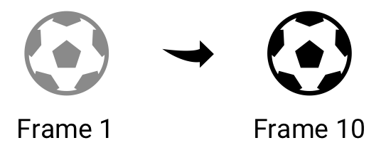
This is a pretty simple calculation, that can be done by comparing the location of the ball at two different times. For example, if the ball at frame 1 is at (0,0) and at frame 10 (now) is at (5,0), it has moved to the right, since the location is translated 5 units along the x-axis.

Implementation-wise, this means that the environment will keep track of the ball’s previous locations. Every time we need to calculate the direction, we look at where the ball was 10 frames ago, and where it is now. We then calculate the change on each axis.

prev = self.history[-10]["position"]
this = self.history[-1]["position"]

dX = prev[0] - this[0]
dY = prev[1] - this[1]

We define a significant movement as a movement of more than 10 pixels, so if the magnitude of dX or dY is greater than 10, there is a movement on that axis. The sign of the number tells us which of way the ball has moved (e.g. we move to the left on the x-axis, if the number is less than zero). If there is a significant movement in both directions, the direction will be of the form ‘DirectionY-DirectionX’, for example: ‘Down-Right’.

Calculate player rotation

Everything we see is from above, so we need a way to calculate rotation. Looking at a picture of the bounding boxes may help us in the right direction:

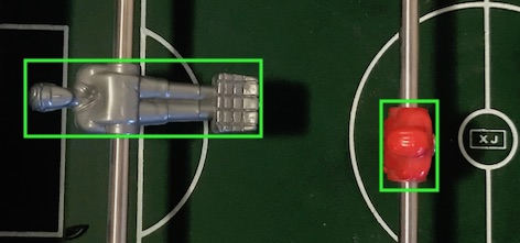
As we can see, a player is rotated if the width of the bounding box is greater than the height, and vice versa. We say that the player is 0% rotated when standing (right player), and 100% rotating when lying (left player). This, however, does not tell us specifically what the ratio should be when the player is 0% or 100% rotated.

One approach to calculate this is to calibrate: we do a full rotation of the row, and the application detects the minimum and the maximum ratios. These will be the 0% and 100%, respectively. However, in my current setup, I don’t want to have to calibrate before playing (after all, it should work for my kids), so I defined the minimum and maximum ratio by trial and error¹.

There is an uncertainty in the approach of using the bounding box: The camera films from a single spot in the middle of the field, so when the players are actually 0% rotated, the camera will detect a slight angle, and believe that they are 10-15% rotated. I am not sure whether this will be a problem, but we will have to see, and eventually revisit this.

Having defined the minimum and maximum ratio, the calculation of the rotation is very simple:

Calculate ball possession

Before we can calculate the ball possession, we need to define what it means to possess the ball. We here propose that a player possesses the ball if it is within the player’s reach. That is, we define an area around the player (the area he can reach), and then we can calculate how much time the ball spends in that area.

We do this by keeping track of which player has possession of the ball in each frame in a ‘possession-table’. For each player, the possession-table will contain the number of frames in which the player possessed the ball. We can then calculate the possession for a player as # frames with possession / # total frames.

We consider the area of reach as a rectangle around the player. We thus need to calculate if the position of the ball is within this rectangle. For each row, we then calculate (for each player) whether the ball is within reach. If so, we increment the possession-table by one for that player.

def calculate_possession(self, ball_position):
    for i, player in enumerate(self.players):
        reach_x_start = player[0] - REACH_WIDTH / 2
        reach_x_end = player[0] + REACH_WIDTH / 2
        reach_y_start = player[1] - REACH_HEIGHT / 2
        reach_y_end = player[1] + REACH_HEIGHT / 2

        ball_x = ball_position[0]
        ball_y = ball_position[1]

         if reach_x_start < ball_x < reach_x_end 
                and reach_y_start < ball_y < reach_y_end:
            self.possession[i] += 1
            break

To calculate team possession, we initialize the game with a configuration of the board, containing information about number of rows, number of players in each row, and the team each row belongs to:

row_config=((3, TEAM_HOME), (3, TEAM_AWAY), (3, TEAM_HOME), (3, TEAM_AWAY))

The team’s possession is then # frames with possession for players in team / # total frames. We now have the possession for both team and players:

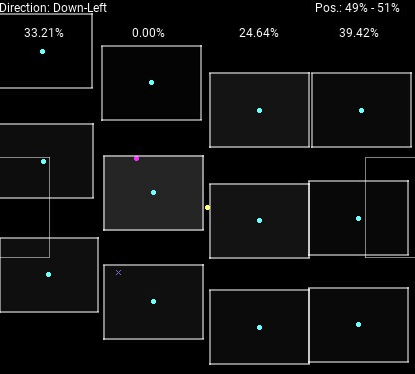
The teams’ possession are shown in the top-right corner, and the each player’s possession is indicated by the opacity of the ‘reach’ rectangle around the player. This visualization also shows the rotation of each row (percentages in the top) and the current direction of the ball.

Detect goals

You may have noticed a small cross in the image above. This actually indicates that a goal was scored from that position. Not only do we detect if a goal has been scored, we also attempt to figure out from which position and by which player.

Inspired by another Table Soccer project, TableSoccerCV, the intuition behind goal detection is to (1) detect that the ball is close to the goal and (2) detect that the ball has now disappeared. If it has disappeared, and was close to the goal, odds are that a goal was scored.

In each game loop, we do as follows:

if ball is in area in front of goal
    check_for_goal <- true
    
if check_for_goal is true
    if ball has disappeared
        increment frames_without_ball by 1
        if frames_without_ball > 15
            GOAL!!  

In other words, when the ball has not been seen for 15 frames (but was seen outside the goal just before), this counts as a goal. The most prominent issue with this, is that it is possible for the ball to be hidden behind or below the goalkeeper. This will result in a false detection of a goal.

When a goal is scored, we then use the history of the ball’s location to figure out the scoring position. We do this by traversing back in history, until the direction of the ball changes. The intuition is that this is the point in time when the shot was performed. It does not work perfectly, e.g. if the ball bounces of another player before entering the goal, but provides an estimate.

We also want to know which specific player scored, so we keep a history of the players’ position together with the ball. When we know from where the goal was scored, we can simply find the player closest to the ball at that time.

for r, row in enumerate(self.player_history[i]):
    for p, player in enumerate(row.get_players()):
        dist = np.linalg.norm(np.array(pos) - np.array(player[0:2]))
        if dist < min_dist:
            min_dist = dist
            player_info["row"] = r
            player_info["position"] = p

Visualization

We now have information about the score, goals and ball possession. Using Flask (as also mentioned in the previous post) we can create a better interface to show and control the application form a browser. We get the current stats using an API endpoint:

@app.route('/stats')
def stats():
    # get data ...
    # ...
    return {
        "score": {"home": score[0], "away": score[1]},
        "possession": {
            "home": team_possession[0], 
            "away": team_possession[1]
        },
        "goals": goals
    }

The web application fetches data from this endpoint every few seconds and populates the model in the webpage. I have chosen to use Knockout.js because of its simplicity and possibility to do declarative bindings, making the implementation of the UI very straightforward. I can simply specify the scores as follows:

<h1 class="display-3" data-bind="with: score">
    Home <span data-bind="text: home"></span> - 
    <span data-bind="text: away"></span> Away
</h1>

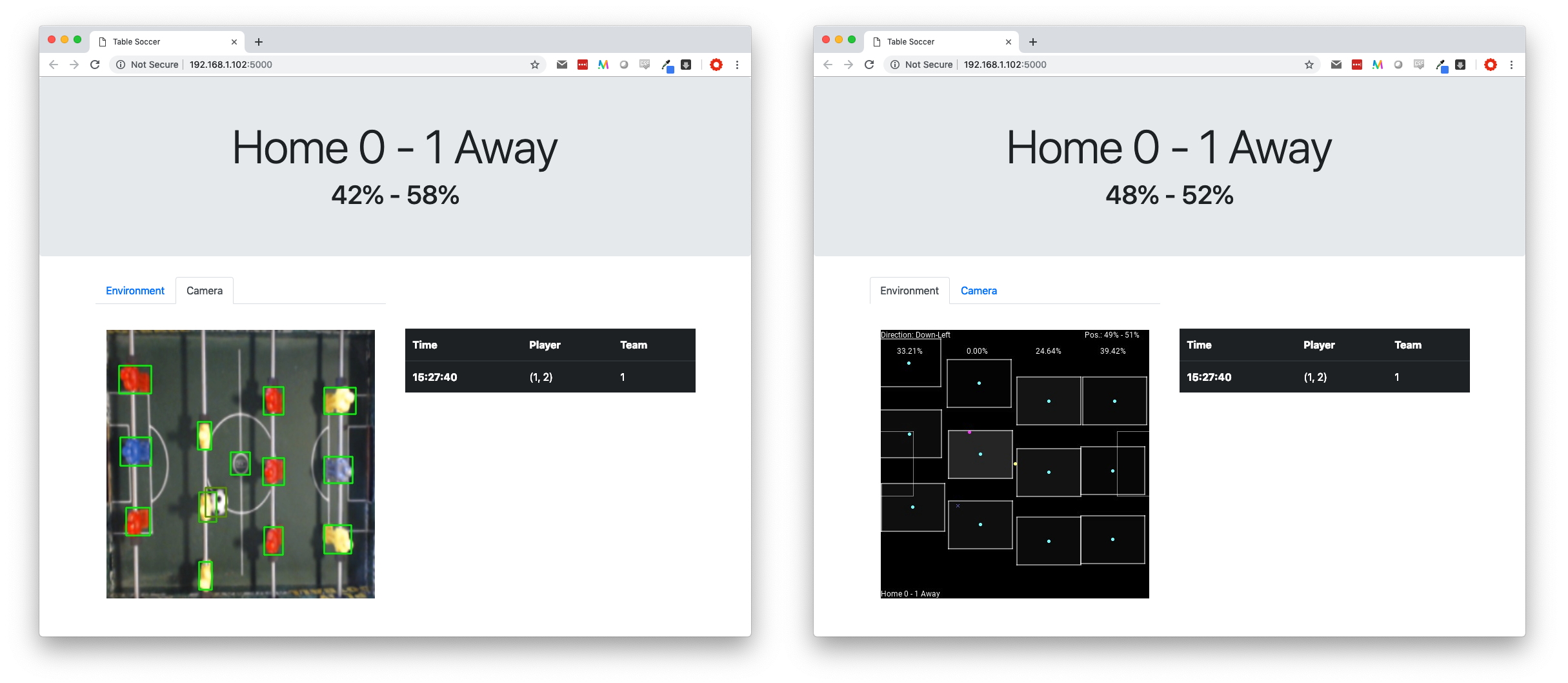
The result is shown below. On the left side, we see the transformed view of the webcam and on the right side, we see the environment representation of the field.

Next steps

Now I can’t postpone it anymore - I am going to start working on the robot. Since I have not worked with hardware much before, the next post will probably be about some of the exploration I am doing in that field.

Footnotes