You Only Look Once!
25 Feb 2019The first real task (now that I have an all-seeing eye) is for my application to be able to understand what it is seeing. As mentioned, I have previously used the OpenCV library to perform the ball-tracking, but it didn’t work too well and I want to track more than just the ball (e.g. the position and rotation of the players). I need some kind of real-time object detection mechanism. There are multiple approaches for this, but currently, the state-of-the-art is YOLO: You Only Look Once. In this post, I will describe what it does and how to measure whether it performs good or bad (i.e. without just looking at the detections). Finally, I show how to use a specific implementation of YOLO to detect objects in a short video clip.
Convolutional Neural Networks
Since this has to do with image analysis, models are usually created using Convolutional Neural Networks (CNNs). This is a subject of its own that I will not dive into here. The main idea is to add convolutional layers to a neural network, which contain a number of learnable filters. During training, the network will learn filters that will activate when detecting certain features in the input. In deep networks, the first convolutional layers typically learn to detect things like edges, while deeper in the network, they will be able to detect more complex features, like an eye or an ear (in the case of images containing faces). The key is that these filters are not pre-defined by the creator of the model, but are learned through training.
By using CNNs, researchers were able to reduce the classification error rate of the ImageNet Challenge significantly by using deep CNNs.
I can highly recommend the Deep Learning specialization on Coursera. In course 4, there is an in-depth explanation of CNNs.
Object Localization
Within the field of image analysis, the objective is often to classify images. This roughly means that we train a model that can tell what a specific image contains (i.e. provide a mapping from an image to one of several predefined categories).
In the figure below, a classification model could classify the image on the left as ‘tablesoccer’. However, for our purpose, we need to know not only that it is a tablesoccer table, but also the location (and rotation) of each player and the ball. This is what is shown in the right image in the figure, where each object is located and a bounding box is drawn around them.
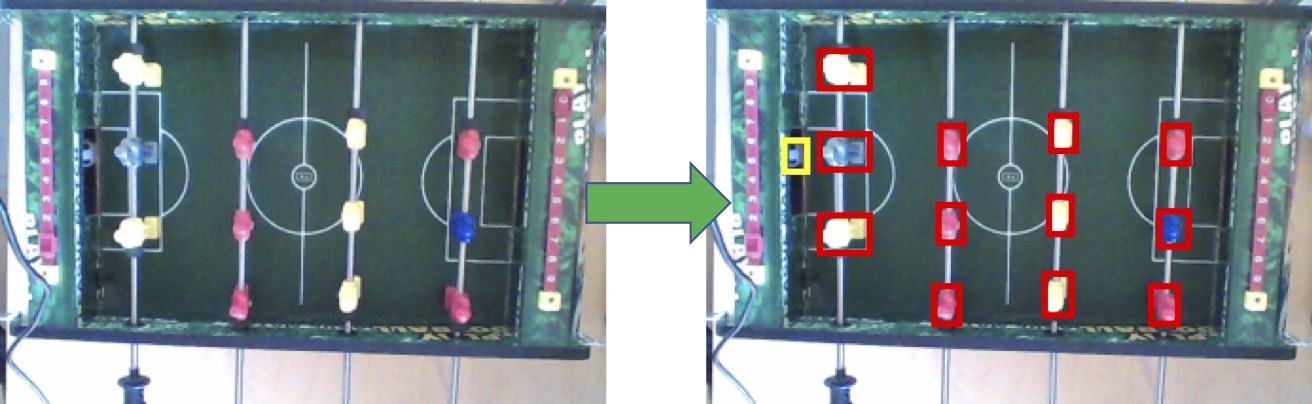
This is a more complex problem, and the output of the localization model is required to contain much more information. Not only do we need to know what was found, we also need information about the bounding box. In classification with $n$ categories, the output, $y$, is a vector of $n$ elements, where each element in the vector is the confidence that the image contains an object in that specific category. For example, if the categories are ‘man’, ‘car’, ‘tree’ and $y = [0.05, 0.85, 0.1]$, then the image most likely contains a car, because the model is 85% confident of this.
Using YOLO, $y$ contains information about the bounding box as well, and thus $y$ contains more information:
\[y = \left[ \begin{matrix} p_c \\ b_x \\ b_y \\ b_h \\ b_w \\ c_1 \\ c_2 \\ c_3 \end{matrix} \right]\]- $p_c$ is 1 if an object is detected, and 0 otherwise.
- $(b_x, b_y)$ is the center of the detected object.
- $b_h$ and $b_w$ are the height and width of the bounding box, respectively.
- $c_n$ is 1 if the object detected is in class $n$.
Note that the output of this model can only locate one object, because it only contains the information of a single bounding box. The output can be extended to include more bounding boxes, making it possible to detect and locate multiple objects in a single image.
Now it is only a matter of doing the actual object localization. A naive approach could be to use brute force: for different sized bounding boxes and at different locations, apply a classification model and select the results with the highest confidence. However, this approach is computationally expensive since it would require many combinations for box sizes and locations to be accurate. YOLO makes it possible to do this in a more efficient way using grids and anchor boxes.
Grids and Anchor Boxes
YOLO breaks an image into grid cells. In a simple setting, it will be possible to detect one object in each cell. Basically, $y$ will be as defined above, but repeated to be able to find one object in each grid cell.
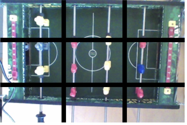
In many cases, it is quite likely to have multiple objects fall into the same grid cell, so this simple version will not be enough. In the figure above, there are multiple players within each grid cell, so we could only locate one of the players within each cell1.
The solution in YOLO is to add anchor boxes. An anchor box is roughly speaking a ‘bounding box template’. Each anchor box will be predefined in a specific shape (e.g. a square, flat rectangle, tall rectangle). The idea is to match the object found in a grid cell to one of these anchor boxes, specifically the one that takes the same shape as the actual bounding box of the object. How well two boxes align can be measured using Intersection over Union (IoU), which I will come back to in the next section.
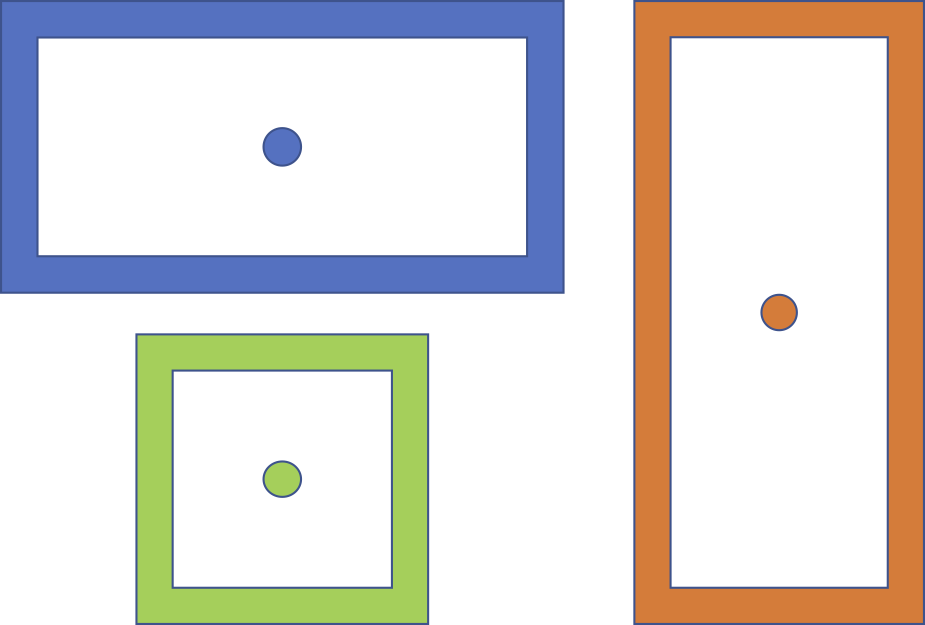
The figure shows example anchor boxes. We could imagine that a standing person will match the tall, red rectangle on the right, while a car will match the flat, blue rectangle.
Anchor boxes are hyperparameters of the model. Hyperparameters, unlike normal parameters, are set before the learning begins. In other words, the model does not learn the best anchor boxes, but we have to supply them. This means that by selecting good anchor boxes, we can get better results. For “The Table Soccer Problem”, the three types of anchor boxes shown in the figure above could match the ball (square box), rotating player (flat rectangle) and blocking player (tall rectangle, but close to a square).
Measuring the performance of the model
Since I’m going to train an existing YOLO model to learn to recognize table soccer objects, I need to know how well it actually performs. To do this, I will calculate the mean Average Precision (mAP) of the model. This is, roughly, the average of model’s precision at different recall values.
In classification, precision is the percentage of predictions made, that were actually correct (the false positive rate). For example, the model predicts that 10 objects are in class $c$, but only 5 of those are actually in that class. The precision is then 50%. Recall is the percentage of actual objects in the class, that the model is able to find (the false negative rate). For example, there are in total 8 objects in class $c$ in the dataset, and the model classifies 6 of them correctly. The recall is then 75%. There will always be a trade-off between precision and recall2.
The average precision for a specific object class can be calculated by finding the precision of the model at a number of recall levels and calculating the average. For example, what is the precision when the recall rate is 50%? Usually, we consider levels 0%, 10%, 20% … 100%. Having calculated the average precision for each class, the mAP is then the average over all the classes.
We can use this to assess the quality of the object detection part of the algorithm. For example, to assess how often the algorithm is able to see that there is a ball, when the ball is actually visible. Since we also need to track the position of the ball, the follow-up question is: how do we measure this when taking the location into account?
Intersection over Union
This is where Intersection over Union (IoU) is used. IoU is a simple formula that measures how much overlap there is between two regions. In other words, we can use it to measure how much overlap there is between the predicted bounding box and the ground truth (the actual location).
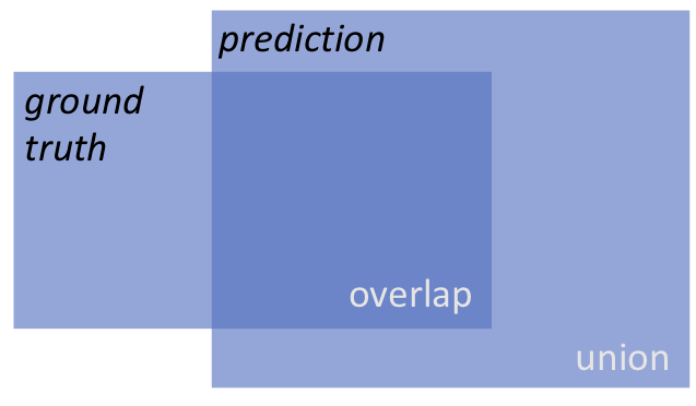
YOLO uses IoU to determine whether or not a specific bounding box is a good candidate for the final output. If the IoU is below a given threshold, the bounding box is suppressed (‘Non-max suppression’). The threshold is often 0.5.
At a given threshold, we can then calculate the mAP. A high threshold will be more strict, since the objects must overlap very much in order to be considered. We would therefore expect a lower number of detections given a higher IoU, but on the other hand also expect that these detections are accurate.
The mAP should be computed from time to time during training, but on the test set. This will help us detect if the algorithm starts overfitting to the training data. This happens when the average loss keeps decreasing, but the mAP is also decreasing. It indicates that the model keeps getting better at predicting from the training set (lower average loss), but is getting worse at predicting from the test set (lower mAP).
Example time!
To test YOLO, I downloaded the Darknet implementation from Github. I use the AlexeyAB-fork which supports Windows. I normally work on Mac, but I have a Windows-machine with an NVIDIA Geforce GPU and I want to be able to use that for the training.
Setup
Configuration and compilation was straightforward: I cloned the repository and followed the ‘How to compile on Windows’ guide.
git clone git@github.com:AlexeyAB/darknet.git
I followed the ‘legacy’ way, since the option to use vcpkg has just recently been supported (after I compiled it). Darknet requires the following tools installed:
- Microsoft Visual Studio: For building the solution.
- CUDA 10.0: The NVIDIA parallel computing platform, to support using the GPU.
- cuDNN 7.4.1: The NVIDIA CUDA Deep Neural Network library for speeding up neural network computations.
- OpenCV 3.X: The Open Source Computer Vision Library. This is the same tool I used for my first rudimentary tracking application.
Having all the requirements installed and configured, building is as simple as opening the build/darknet/darknet.sln file and building the Release version for x64. The result is the darknet executable, which contains all the YOLO functionality.
Running a simple example
I downloaded weights for Yolov3. That is, a file that contains the final weights for a fully trained model using the Yolo architecture. The model is trained on the ‘Common Objects in Context’ (COCO) dataset.
I first tried to use the detector for a picture of a dog that comes with the Darknet repository:
darknet.exe detector test data/coco.data yolov3.cfg yolov3.weights -i 0 -thresh 0.25 dog.jpg -ext_output
And voila:
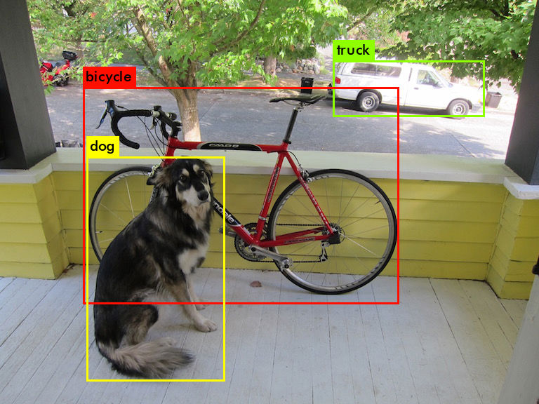
It was very satisfying to see that the setup and compilation went so smoothly, as I have often experienced quirks when compiling specialized software.
Real-time video processing
Finally, I wanted to test the performance when doing real-time predictions on a video. The repository comes with a Python-implementation that uses Darknet as a library (DLL in the Windows case). To use this, I first had to build the DLL (by building the build/darknet/yolo_cpp_dll.sln project). Then it is possible to run detections from Python:
from darknet import performDetect

result = performDetect(image, makeImageOnly=True, configPath=config, weightPath=weights, metaPath=data)
The result is a dictionary containing all the found bounding boxes and (if makeImageOnly is true, return the image with the bounding boxes drawn). I had to make some small adjustments because I ran into some errors when loading the class names (this commit).
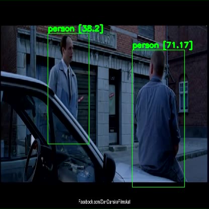
I downloaded a clip from YouTube and processed it using the full Yolov3 model. The clip is 2 minutes and the processing took 147 seconds. An excerpt of the result is shown here:
It is detecting people with very high confidence (almost always > 95%). It also detects a tie, a car and some other things (also a TV monitor, even though there isn’t one).
Since the processing time exceeded the length of the clip, it seems that the full Yolo architecture may be too large for our purposes. We require real-time processing to be able to detect the ball and react immediately. To do this, we can try to use the tiny version of Yolo, which contains fewer layers and therefore requires significantly fewer operations for each image.
Using the tiny version, I was able to process the entire clip in only 52 seconds. As a result (and as expected) the quality of the predictions is also significantly lower. Here, the two persons are detected, but the car is not, and the confidence is quite low compared to the full model.
Given the speed-up from Yolo to Yolo-Tiny, I hope to be able to use the tiny version. Since my domain is much smaller with fewer classes and an environment that does not change much, it seems plausible that even a not-so-deep architecture could perform pretty well.
Next step
I now have Darknet up and running and can perform object localization using pre-trained models. The next step is to create a model that can be used for locating the players and the ball in tablesoccer!
External links
- Deep Learning on Coursera
- Deep Learning: Course 4
- Anchor Boxes — The key to quality object detection